Click on a header on the header panel above to get directed to the main sections of this documentation

To navigate through more specific sections of this documentation, scroll through the grey navigation panel present at the right side of this page and click on a header.

To get a quick idea of how you can select the most relevant results from ORVAL, click on the Tutorials header above.

Summary

ORVAL is the first web bioinformatics platform for the exploration of predicted candidate disease-causing variant combinations, aiming to aid in uncovering the causes of oligogenic diseases (i.e. diseases caused by variants in a small number of genes). This tool integrates innovative machine learning methods for combinatorial variant pathogenicity prediction, further external annotations and interactive and exploratory visualisation techniques.

What can you do with ORVAL?

SUBMIT AND FILTER YOUR VARIANTS

You can submit the variants of a single individual either as a variant list or a VCF file.
You can also filter your variants based on their Minor Allele Frequency (MAF), their position in the gene and/or based on a specific gene panel of your choice.

PREDICT CANDIDATE DISEASE-CAUSING VARIANT COMBINATIONS

With ORVAL you can predict candidate pathogenic variant combinations in any gene pair present in your data with VarCoPP and further predict their digenic effect (True Digenic, Monogenic with a Modifier variant or Dual Diagnosis) with the Digenic Effect Predictor.

EXPLORE POTENTIAL OLIGOGENIC SIGNATURES

You can investigate potential oligogenic disease signatures by exploring the interactive gene networks that are created based on the predictions and examine them in the context of their protein-protein interactions, cellular locations and pathways.

NOTE: The main results of this platform are based on predictive tools. They are provided for research, educational and informational purposes only and the pathogenicity predictions should be subject to further scientific and clinical investigation.
It is not in any way intended to be used as a substitute for professional medical advice, diagnosis, treatment or care.

The input data

ORVAL accepts a list of variants from a single individual only, as it creates all possible variant combinations between pairs assuming that these belong to the same individual.

You can provide either Single Nucleotide Variants (SNVs) or small insertions/deletions (indels).

NOTE: The use of ORVAL for the analysis of complete patient exomes is NOT recommended, as our methods are not fine-tuned for exomes. Please restrict your analysis to relevant gene panels for the disease of interest. If your VCF contains the complete exome of an individual, you can upload it in ORVAL as it is, and then use the Variant Filtering and Gene Filtering options before submitting your data.

Types of input files

There are two different types of variant input that you can use to upload your data: either a variant list or a VCF file. After uploading your data, you can start the analysis by clicking on the button.

Tab-delimited variant list

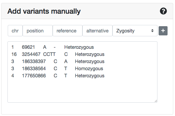
At the left panel of the Submit variants page you can insert/copy-paste a variant list. Each line should contain tab- or space-delimited information for one variant, in the corresponding order: chromosome, position, reference allele, alternative allele, zygosity.

No headers are needed.

The zygosity values should be either Heterozygous or Homozygous. During the analysis, ORVAL automatically converts X-linked variants in males as Hemizygous.

You can also manually insert a variant in this list by typing information:

at the next line and making sure that you use the same delimiter for all columns
at the corresponding chr, position, reference allele, alternative allele, Zygosity column fields and pressing the button.

NOTE: using the variant list panel, you can upload up to 80000 variants.

VCF file

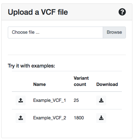
Alternatively, you can submit a VCF file (version 4.2) with your variants at the right panel of the submission page.

ORVAL requires as minimum the presence of:

the #Header Line: #CHROM POS ID REF ALT etc... line
the columns CHROM, POS, ID, REF, ALT, FORMAT, SAMPLE_NAME (patient information column containing values corresponding to the FORMAT field).
the genotype (GT) field for each variant at the FORMAT and SAMPLE_NAME columns. We use GT to define the zygosity of the variant and to pick the correct alternative allele if there are multiple ones (separated by commas) in ALT.
In case variants with GT: 0/0 ; 0|0 ; ./. ; . are present, these are discarded from the analysis. Allele combinations only consisting of alternative alleles (e.g. GT: 1/2 or 3/2) are handled as two separate heterozygous variants.

Any other meta-information lines on the top of the file or any extra columns and fields (e.g. QUAL, INFO, etc.) can be present, but ORVAL will ignore them.

NOTE: if your VCF contains information for several individuals, you should separate the information of each individual in different VCF files and run them individually in ORVAL.

NOTE: you can upload a VCF file of size up to 50 MB. The file can also be compressed either with zip, gzip, bzip2 or xz.

In case you want to create your own VCF file, you can download and take a look at the example VCFs that are present at the VCF submission panel and/or consult the Samtools specification page on how to construct a proper VCF file.

Variant types

You can either submit Single Nucleotide Variants (SNVs) or small insertions/deletions (indels). Other types of variants (e.g. CNVs) can be present in your list, but they will not be included in the analysis.

Specifically for indels, you can submit your variants in either one of the two different ways that are shown for a particular variant example (the VCF file can contain more columns).

	Tab-delimited list	VCF file
Example with dashes	16 3254468 CTT - Heterozygous	16 3254468 . CTT - PASS GT 1/0
Example without dashes	16 3254467 CCTT C Heterozygous	16 3254467 . CCTT C PASS GT 1/0

Genome version

At the moment ORVAL accepts and annotates variants using either the GRCh37/hg19 or the GRCh38/hg38 human genome assembly.

We do not make conversions of genomic coordinates from different genome versions. In case you need to convert your variants, you are encouraged to use tools like the UCSC, Ensembl and NCBI assembly converters.

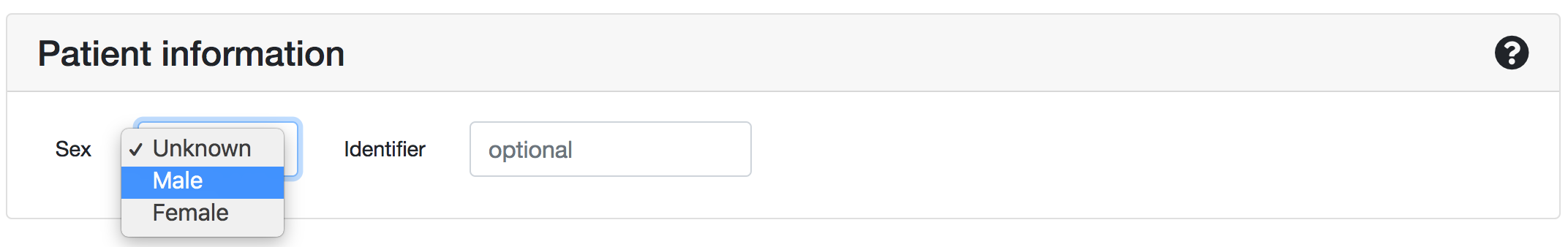
Patient information

Except from the variant list, you should also provide (if available) the sex information of the patient, i.e. if the person is a male or a female.

ORVAL handles differently X-linked variants in males (hemizygous variants) compared to females, and therefore this information is important in order to provide better predictions.

Example input files

You can try ORVAL with the two example VCF files that are present in the VCF file section of the variant submission page (for both genome assemblies). These files give you the opportunity to test ORVAL on a small or large number of variants and see what the webserver has to offer.

the Example_VCF_1 file contains 25 variants.
the Example_VCF_2 file contains 1800 variants.

Job submission

Every time you submit your data, you will first get directed to the Submitted ORVAL Job page where you can follow the status of your submission.

In this page you will also receive a Job Id, which you can use to re-access the results of that specific submission or report errors. That Job Id is also present in the Results site in the format: orval.ibsquare.be/results?id=YourJobID.

You can re-access your results by:

saving the URL of the Job or the Results page
typing on your browser https://orval.ibsquare.be/results?id= followed by the Job ID

Do you receive error or warning messages during your data submission? You can consult the Frequently Asked Questions (FAQ) section for suggestions on how to handle them.

NOTE: all result information is automatically deleted 7 days after the submission at 04.00 am (GMT+2). After this period, you have to re-submit your data and you will receive a new Job Id.

NOTE: for server monitoring purposes we allow every user (based on their IP address) to run up to 5 different Submission Jobs at the same time. In case you exceed this number, you will have to wait until at least one of the running Jobs is finished to launch a new one.

Data filtering and annotation

Data filtering

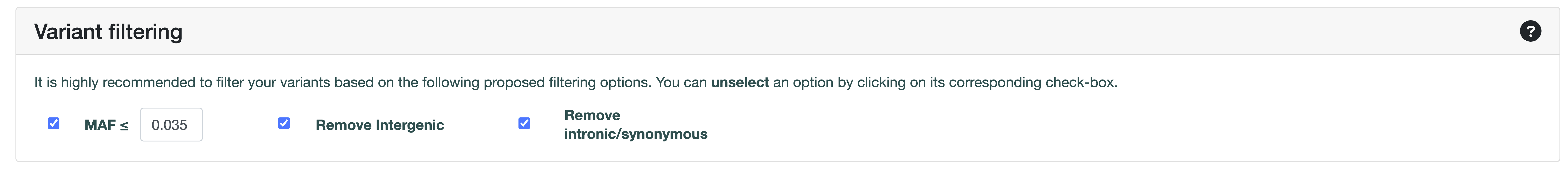
In the Submit variants page, ORVAL offers a recommended variant and gene filtering procedure that will automatically run when you submit your data. This procedure is highly recommended, as it will limit the amount of variant combinations to be tested and will restrict the analysis to the most relevant variants.

There are two types of filtering offered by ORVAL: a variant filtering and a gene filtering procedure.

Variant filtering

The variant filtering procedure ensures that your analysis will contain variants in accordance with the variant types used to train the predictive methods (VarCoPP and Digenic Effect predictor) integrated in ORVAL: exonic and splicing variants of MAF lower or equal than 3.5% in protein-coding genes.

The three different filtering options are already pre-selected in the Variant Filtering panel of the submission page. You can unselect a filtering option, by clicking on its corresponding check-box.

Filtering options

MAF

Select the minimum threshold of MAF for the variants. A MAF of ≤ 0.035 was used to train VarCoPP and is the recommended threshold.

Remove Intergenic

Removes variants that are not inside the defined gene coordinates, based on the selected assembly (GRCh37/hg19 or GRCh38/hg38).

Remove intronic and synonymous

Removes:

all intronic variants that have a distance bigger than 13 nucleotides from each exon edge, based on the exon coordinates of the canonical transcript of the gene.
all synonymous variants that have a distance bigger than 195 nucleotides from each exon edge, based on the exon coordinates of the canonical transcript of the gene.

NOTE: apart from the requested filtering steps, ORVAL may also exclude some extra variants during the data annotation process. You can consult the complete list of variant exclusion cases during that process here.

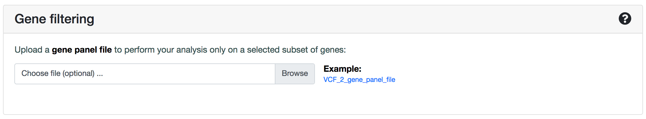
Gene filtering

The gene filtering option restricts the analysis to a specified list of relevant genes that can be present in your data. This procedure is highly recommended in case your VCF contains the complete exome of an individual, as it can dramatically limit the amount of False Positives that can be obtained.

To run your analysis only with a subset of genes, you can simply upload a .txt file with the genes you are interested to include, each gene being in a different line. You can submit ENSGs or gene names. After submission, ORVAL will use this list to filter the genes that will be used in the analysis.

NOTE: please make sure that you provide the official approved symbol or ENSG for each gene (for verification, you can consult the HGNC gene nomenclature page or the Ensembl genome browser.

Data annotation

After you submit your data, ORVAL:

automatically annotates them with the biological information (list of sources and current versions in the link) needed for the integrated predictive methods (VarCoPP and the Digenic Effect predictor)
creates all possible variant combinations between any pair of genes present in your variant input and
orders the variants and genes inside each combination.

Below, you can find some important parameters for each process.

Gene annotation

To map variants in genes, ORVAL uses at first the gene information that is present in the CADD annotation file for that variant and uses only the canonical transcripts of those genes, according to the Ensembl GRCh37/hg19 or GRCh38/hg38 genome version.

In cases where a variant can be mapped to multiple genes, ORVAL maps that variant to only one gene based on a set of priority rules that include (starting from higher to lower priority): valid gene IDs and canonical transcript, prioritisation of genes based on their biotype and the functional consequence of the variant, prioritisation of genes where the variant falls inside the gene and canonical transcript coordinates, presence of a CCDS, prioritisation of gene with the longest canonical transcript, etc.

ORVAL then annotates the genes with:

the required gene features for VarCoPP (detailed description of the features and their sources in the link)
the required gene features for the Digenic Effect predictor (detailed description of the features and their sources in the link)
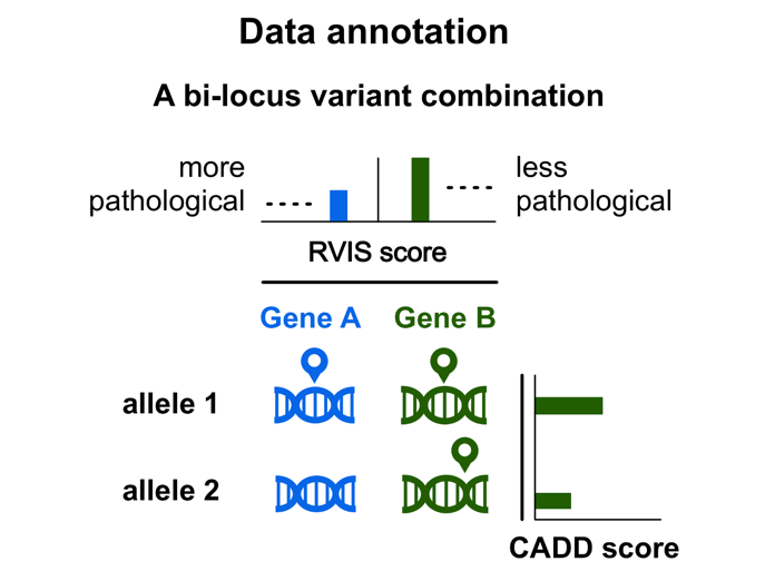
the Residual Variation Intolerance Score (RVIS), a metric that show the susceptibility of a gene to disease. Lower values of RVIS indicate greater susceptibility of a gene to candidate disease-causing mutations.
the protein sequences from Uniprot using the Ensembl canonical identifiers, as these are needed to calculate some of the features of our predictive methods

Gene pair annotation

ORVAL annotates a gene pair with:

the gene pair features required by VarCoPP (detailed description of the features and their sources in the link).
involvement in the same pathway information from Reactome, which is used as a feature for the Digenic Effect predictor
protein-protein interaction (PPI) and cell co-localisation information from the comPPI database

ORVAL uses the Residual Variation Intolerance Score (RVIS) metric to order the appearance of genes inside each digenic variant combination, with gene A being always the gene with the lower RVIS value, and thus more probable to be have a disturbed function due to the presence of a variant. You can find more details about how ORVAL creates digenic variant combinations and orders variants and genes in the Creating digenic variant combinations section of the Documentation page.

Variant annotation

ORVAL first maps a variant in a gene based on the Gene annotation process described above. It then annotates each variant with:

the required variant features for VarCoPP, the most important being the CADD score (detailed description of the features and their sources in the link)
the required variant features for the Digenic Effect predictor (detailed description of the features and their sources in the link)

When ORVAL creates digenic variant combinations, it uses the CADD score to order the appearance of variants that are present inside the same gene (i.e. in cases of heterozygous compound variants). You can find more details about how ORVAL creates digenic variant combinations and orders variants and genes in the Creating digenic variant combinations section of the Documentation page.

Variant exclusion

In some situations during the data annotation process ORVAL excludes variants from the analysis and you will not find them in the results:

Variant not exonic in canonical transcript
We use only the canonical Ensembl transcript identifiers to annotate our variants. If you have selected to exclude intronic variants from your analysis, if the variant is not exonic in the canonical transcript of the gene, even if it may be exonic in an alternative transcript, it will be excluded.
Variant with invalid zygosity
Variants with GT:0/0 or GT:0|0 in a VCF file are considered invalid and are excluded from the analysis.
CADD score not available
ORVAL annotates variants with a CADD score, which is a feature required for the pathogenicity predictions. As this feature is important for the predictions, if a CADD score is not available for a variant, that variant is excluded for the analysis, as a missing value may severely alter the results.
Variants only in one gene
As ORVAL creates combinations between gene pairs, if your input data includes variants from one gene only, you will not get any results.
The variant is a CNV or medium/long-sized InDel
ORVAL analyses only SNVs and small insertions and deletions (up to 100 bp currently). Any other variant type in your data is automatically excluded from the analysis. This is mainly due to the computational resource limitations of our service.

Creating digenic variant combinations

After annotation, VarCoPP creates all possible variant combinations between any gene pair present in your input, taking into consideration any filtering options you have included during your variant submission.

You can find below a list of details and constraints that take place during this procedure.

Number of variants per combination

ORVAL creates for any gene pair variant combinations that can be:

bi-allelic (i.e. one mutated allele at each gene)
e.g.: one heterozygous variant per gene

tri-allelic (i.e. three mutated alleles in total)
e.g.: an homozygous variant at gene A and an heterozygous variant in gene B

tetra-allelic (i.e. four mutated alleles in total)
e.g.: one homozygous variant per gene

In the tri-allelic and tetra-allelic cases, a digenic combination can also include heterozygous compound variants (i.e. two different mutated alleles in the same gene), along with the presence of variant(s) in another gene.

NOTE: Tetra-allelic variant combinations with heterozygous compound variants in BOTH genes are not created.

NOTE: In case where multiple heterozygous variants are present in a single gene, these are used together as heterozygous compound variants in a combination with another gene and not individually anymore. This is to solve the problem of certain genes being over-represented in the results just because they contain heterozygous compound variants.
If a single gene contains more than two heterozygous variants, these are used in pairs of two as we always use two mutated alleles per gene.

Order of genes

For each digenic variant combination, gene A is always the gene with the lowest Residual Variation Intolerance Score (RVIS) (see also the Gene Annotation section) and, thus, the one with a higher probability to be associated with a disease.

Order of variant alleles inside the gene

In case of two different mutated alleles in the same gene (heterozygous compound cases), the variant allele 1 is always the variant allele with the highest CADD score.

A graphical representation of a digenic combination

The predictive methods of ORVAL

VarCoPP: the variant combination pathogenicity predictor

VarCoPP stands for Variant Combination Pathogenicity Predictor. It is a machine-learning method that predicts the pathogenicity of any bi-locus variant combination (i.e. a combination of two to four variant alleles between two genes).

The method has been published in the PNAS journal: https://doi.org/10.1073/pnas.1815601116. The first version of the model was later improved to VarCoPP2.0 using new training data, new features and a different type of model. VarCoPP2.0 has been published in BMC Bioinformatics: https://doi.org/10.1186/s12859-023-05291-3. See also the Cite us section in the About page, for a list of all relevant citations.

Based on VarCoPP, a bi-locus variant combination can either be candidate disease-causing or neutral.

VarCoPP has been trained separately for the GRCh37/hg19 and GRCh38/hg38 genome assembly, the correct model will run based on your assembly choice in the Input section.

Structure of VarCoPP

ALGORITHM

VarCoPP2.0 is a Balanced Random Forest (RF) predictor that consists of 400 decision trees.

TRAINING DATA

The VarCoPP2.0 predictor has been trained on the pathogenic variant combinations present in the Oligogenic Diseases Database (OLIDA) against a large subset of variant data derived from control individuals of the 1000 Genomes Project (1KGP).

The variant types that were used for training were the same for both OLIDA and 1KGP: exonic and splicing variants of up to 3.5% MAF, while all genes were protein coding genes.

RESULT CALCULATION

VarCoPP2.0 outputs a VarCoPP score, i.e. the probability (value between 0 and 1) that a variant combination belongs to the disease-causing class. If this probability is above 0.50 (hg19) or 0.4575 (hg38), the model predicts that the combination is disease-causing.

Prediction features

VarCoPP uses different variant, genes and gene pairs biological features to make the predictions.

Feature	Source	Feature abbreviation	Gene / Variant allele
CADD raw score PMID: 24487276	CADD v1.6	CADD1 CADD2 CADD3 CADD4	Gene A / Variant allele 1 Gene A / Variant allele 2 Gene B / Variant allele 1 Gene B / Variant allele 2
Gene haploinsufficiency prediction PMID: 28137713	dbNSFP v4.1	HIPred_A HIPred_B	Gene A Gene B
Inheritance specific pathogenicity prediction for autosomal dominant (AD), autosomal recessive (AR), and X-linked (XL) modes of inheritance PMID: 27354691	publication supplementary data	ISPP_AD_A ISPP_AD_B ISPP_AR_A ISPP_AR_B ISPP_XL_A	Gene A Gene B Gene A Gene B Gene A
Selective pressure (dN/dS) PMID: 26896847	Ensembl v99	dN_dS_A	Gene A
Biological distance PMID: 24694260	Human Gene Connectome v12.2015	Biol_Dist	Gene pair AB
Biological Process similarity PMID: 10802651, 18460186	Gene Ontology v2021-12	BP_sim	Gene pair AB
Distance in an in-house developed Knowledge Graph PMID: 37644440	BOCK v1.0	KG_dist	Gene pair AB

99% and 99.9% confidence zones

With VarCoPP2.0 we have defined 99% and 99.9%confidence zones, delimited by the prediction threshold, which provide a probability of whether a particular combination predicted as candidate disease-causing, is actually a True Positive (TP) result. This indication can be useful for further evaluation and filtering of the predictions.

These confidence zones were created by testing neutral bi-locus combinations from the 1000 Genomes Project and obtaining the minimal prediction probability that gave 1% and 0.1% False Positives respectively. If a combination falls into either one of the two zones, a coloured indication will appear in the summary results.

99%-confidence zone

Requires VarCoPP score ≥ 0.743 (hg19) or ≥ 0.647 (hg38). If a digenic combination falls inside this zone, it has 99% probability of being a TP result.

99.9%-confidence zone

Requires VarCoPP score ≥ 0.891 (hg19) or ≥ 0.85 (hg38). If a digenic combination falls inside this zone, it has 99.9% probability of being a TP result.

The Digenic Effect Predictor

The Digenic Effect predictor is a machine-learning method that predicts the type, or else the digenic effect of a pathogenic digenic variant combination. This information could be useful in case there is no pedigree information or parent genotypes available, as it could give a predictive indication of the effect of a predicted as pathogenic variant combination. As this is a machine-learning approach, again, a manual investigation by the user can confirm or reject the assigned digenic effect class.

The Digenic Effect predictor has been published in the Artificial Intelligence in Medicine journal: https://doi.org/10.1016/j.artmed.2019.06.006 and the Nucleic Acids Research journal: https://doi.org/10.1093/nar/gkx557. See also the Cite us section in the About page, for a list of all relevant citations.

IMPORTANT UPDATE: An update of the Digenic Effect predictor has been made using up-to-date versions of all required features (check the Updates page). This means that the obtained results may differ than those from the corresponding publication.

The Digenic Effect predictor can distinguish between three classes of pathogenic variant combinations:

True Digenic

Variants at both genes are needed to show the disease phenotype.

Monogenic + Modifier

The variant at the first gene acts as the major monogenic variant that can trigger disease symptoms, while the second variant acts as a modifier of symptoms severity or age of onset.

Dual Molecular Diagnosis

Conjunction of variants that trigger two independent monogenic disorders that occur simultaneously within a single patient.

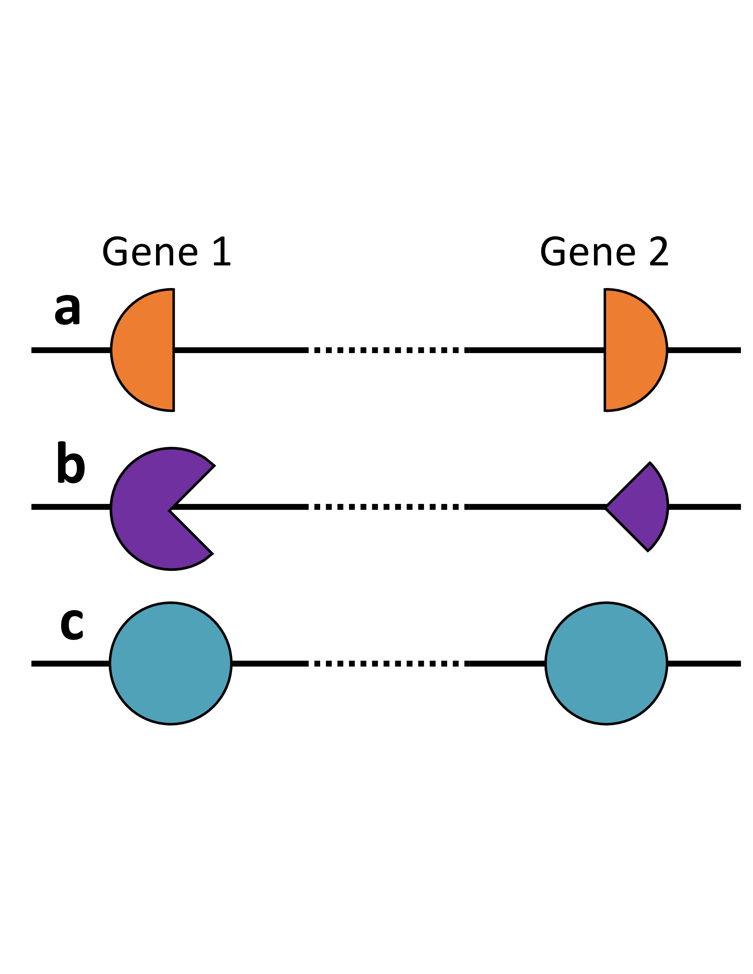
The three types of digenic effects.
Combination a, a True Digenic combination, where the simultaneous presence of a pathogenic allele in each gene is necessary for the individual to express the disease. phenotype.
Combination b, a Monogenic plus Modifier combination, where a variant on the major gene induces a disease phenotype, while a mutation in the modifier gene modifies it, either by rendering it more severe or producing an early onset.
Combination c, a Dual Molecular Diagnosis combination, where both loci are responsible for either distinct or overlapping phenotypes for two different diseases.

The structure of the Digenic Effect predictor

ALGORITHM

The Digenic Effect predictor is a classification Random Forest (RF) algorithm.

TRAINING DATA

The Digenic Effect predictor was trained on 240 pathogenic variant combinations.

More specifically, it has been trained on 90 True Digenic and 75 Monogenic+Modifier variant combinations present in the Digenic Diseases Database (DIDA) and 75 Dual Molecular Diagnosis combinations derived from the work of Posey et al.

The variant types were single nucleotide variations and small insertions/deletions.

RESULT CALCULATION

The Digenic Effect predictor provides probabilities (from 0 to 1) for all three digenic effect classes for a variant combination.

The final digenic effect class is the class with the highest probability among the three.

Prediction features

The Digenic Effect predictor uses different variant, genes and gene pairs biological features to make the predictions.

Feature	Feature abbreviation	Gene / Variant allele
CADD raw score PMID: 24487276	CADD1 CADD2 CADD3 CADD4	GeneA / Variant allele 1 Gene A / Variant allele 2 Gene B / Variant allele 1 Gene B / Variant allele 2
Gene recessiveness probability PMID: 22344438	RecA RecB	Gene A Gene B
Essential in mouse PMID: 23675308	EssA EssB	Gene A Gene B
Same pathway SOURCE: Reactome	Pathway	Gene pair AB

Navigation of the ORVAL results

After the analysis is finished, you will be directed to the Results page, where you will find an expandable job summary at the top. In the subsequent parts, you can explore the oligogenic network that is created using the VarCoPP predictions, the ranking of your gene pairs, based on their content of predicted candidate disease-causing combinations and the detailed digenic pathogenicity probabilities and scores information of your input.

You can access each section by clicking on the corresponding tab at the navigation bar at the top of the page.

NOTE: you can re-access the results of your input for 7 days by bookmarking the Job or Results page of your submission.

Job summary

The Job summary shows the information that you submitted in the Input page: the ID and Sex of the patient, the filtering settings and the variant input. It also shows how many of your variants remained after the filtering and annotation (and were used for predictions).

By clicking on "Details...", you can display a breakdown of the discarded variants. It shows how many variants had an invalid zygosity, were filtered out, or had a missing CADD score. For each of those categories, it is possible to download a list of the variants in .txt file.

If you can share your variant data, don't hesitate to send us the variants with missing CADD score so that we can try to add them to our database.

Oligogenic exploration

This section provides the space for the exploration of potentially oligogenic signatures. The information is guided by the predictions of VarCoPP, which predicts the pathogenicity of variant combinations between gene pairs.

The oligogenic information is mainly shown in the form of a gene network, whose nodes represent genes and whose edges connect two genes only if there exists at least one variant combination between them that has been predicted as candidate disease-causing with VarCoPP. The users can explore and filter the network, as well as investigate the protein-protein interactions and the involved pathways of the genes that belong in the same module.

Oligogenic combination network

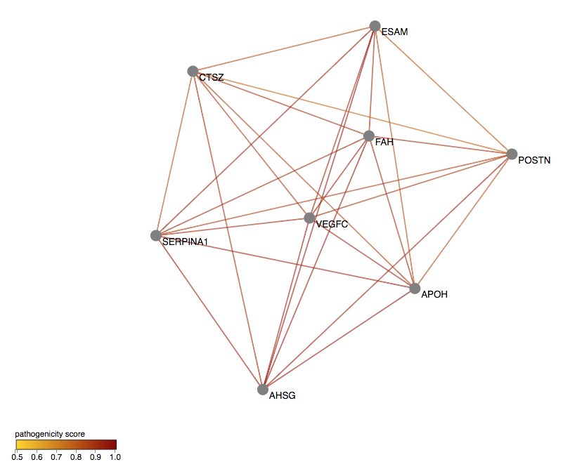
The first panel of the main Results page, contains the predicted candidate disease-causing oligogenic combination network.

Network description

Like every network, the oligogenic combination network contains nodes and edges.

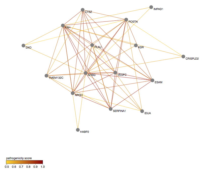
Node

Each node represents a gene present in your data.

Edge

Connects two genes only if there exists at least one candidate disease-causing variant combination predicted by VarCoPP between them.

The colour of the edge represents the highest pathogenicity score for that pair.
This score is represented in a colour range from yellow (low pathogenicity score) to dark red (high pathogenicity score), representing scores from 0.49 to 1.0, respectively.

You can:

Move a node
You can select and move a node to arrange it in the network.
Click on a node
By clicking on a node, this node appears with a purple border and a module panel appears automatically on the right of the panel with more information about the module the gene belongs to. At the top of that module panel, the Click here to further explore this gene module link directs you to the specialised page for your selected oligogenic module.
Download the network
By clicking on the download button, which is present at the bottom right of the panel, you can download the network in its current state, including the filtering options you have selected, in the Graph ML format. This file format can be imported in various graphical tools, e.g. with yED or in network analysis tools, such as Cytoscape and and Gephi.

NOTE: gene pairs with only neutral variant combinations are excluded in this section, and this means that a proportion of your input data and of the digenic results may not be present in the network. You can nevertheless see the predictions for all combinations in the Digenic Predictions section.

NOTE: if you select to download the oligogenic network, this will include any filtering options you have selected (removing genes or edges). Therefore, if you want to download the complete initial network, you should de-select all your filtering options.

Gene selection

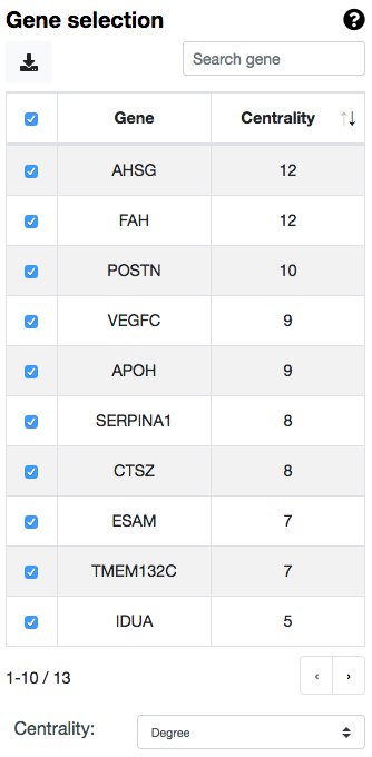
The Gene selection table on the left of the panel contains all genes present in the oligogenic network. The gene table changes automatically according to the filters you select either on the table itself or on the Filtering section below.

At the beginning, all genes are automatically selected and shown in the network.

You can:

remove a gene from the network by clicking on its corresponding check box and unselecting it.
order the appearance of genes based on their centrality in the network, and this centrality can be based either on the:
- degree of the node: the number of edges connected with that node
- closeness of the node: the sum of the length of the shortest paths between the node and all other nodes in the graph, i.e. how close the node is with the other nodes of the network
click on a gene to show the module panel with more information about the gene module it belongs to.
search the table based on a gene name.
download the table in its current state with the button.

NOTE: if you select to download the gene selection table while you have unselected genes or other filters active, only that filtered table will be downloaded. Therefore, if you want to download the complete table, you should make sure that all genes are selected and all filters are reset to default settings.

Network filtering

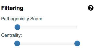
The network filtering option allows you to remove edges from the network by adjusting the thresholds of two metrics:

the pathogenicity score: the threshold for the highest pathogenicity score for a combination of a gene pair, which is based on the VarCoPP score (see the VarCoPP section for more details)
the centrality: the centrality threshold of a gene in the network

Oligogenic gene module

In this section you can further explore and filter the genes of your selected gene module, with the oligogenic gene module network on the right and the module gene selection table on the left of the panel.

The oligogenic gene module network description

This is the selected gene sub-network shown in the exact same way that is present in your main oligogenic network. The nodes and edges of the network represent, again, the genes and the highest VarCoPP Scores of the gene pairs, respectively (see the Oligogenic Network section for a description).

example of a selected gene module from the oligogenic network

You can:

Move a node
You can select and move a node to arrange it in the network.
Download the module
By clicking on the download button, which is present at the bottom right of the panel, you can download the gene module in its current state, in the GraphML format. This file format can be imported in various graphical tools, e.g. with yED or in network analysis tools, such as Cytoscape and and Gephi.

Module gene selection

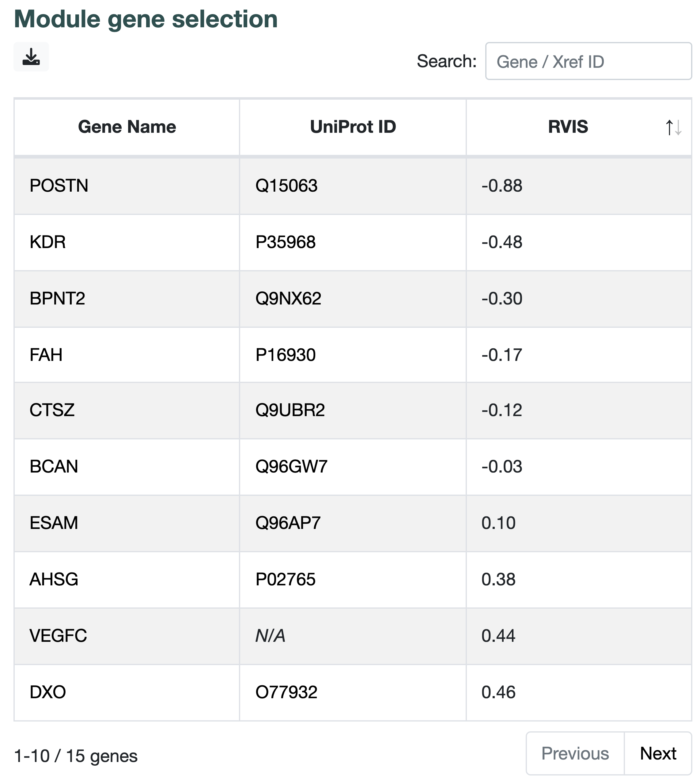
The Module gene selection table on the left of the page contains all the genes present in your selected oligogenic module.

You can:

search a gene on the table based on its name or external ID (e.g. Ensembl or Uniprot ID).
order the appearance of the genes based on their Residual Variation Intolerance Score (RVIS), with genes having a lower RVIS being more probable to carry pathogenic mutations.
click on a gene name to be directed to its corresponding HGNC page.
click on an external ID to be directed to its corresponding source page.
download the table in its current state with the button.

NOTE: if you select to download the module selection table while you have an active gene search, only the information about that gene will be downloaded. Therefore, if you want to download the complete table, you should make sure that the search field of the table is empty.

Protein-protein interaction information

In this section you can explore any existing direct and indirect protein-protein interactions (PPIs) present in your selected module and get information about the position of the proteins in the cell.

All required information is extracted from the comPPI database.

Protein-protein interaction network

On the left panel of this section you can see a protein-protein interaction network that contains nodes and edges.

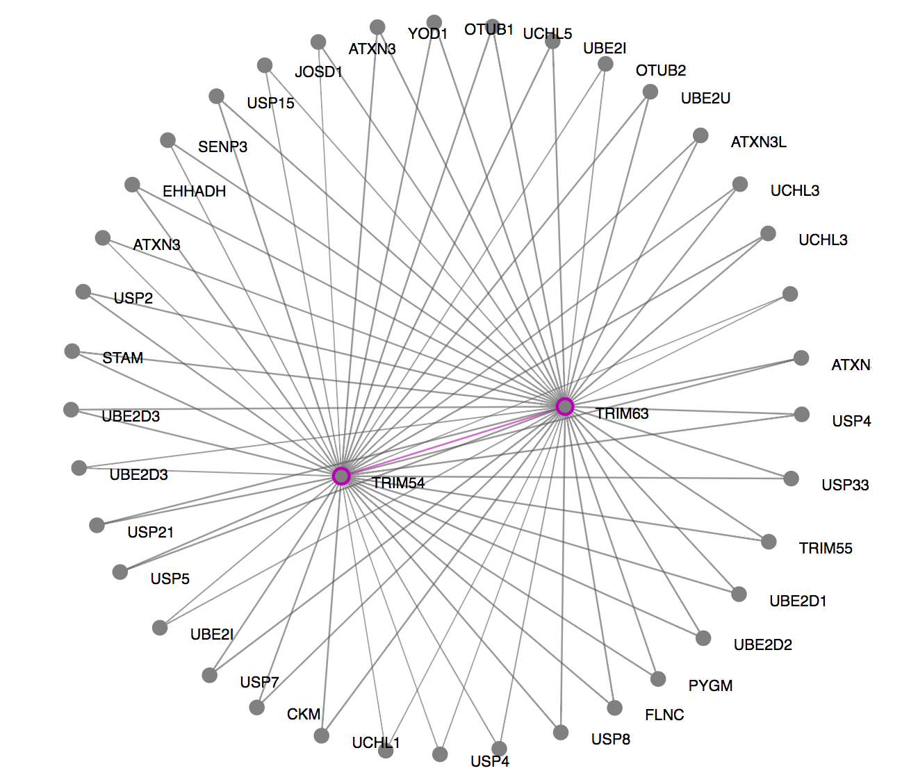
Node

Each node represents a protein.

There are two types of nodes in this network:

Purple nodes: the proteins of your selected module
Grey nodes: external proteins that are present in the network only if they directly interact with two proteins of the selected module. These proteins are useful to show indirect physical interactions of your selected proteins.

Edge

Connects two nodes (proteins) if they directly physically interact.

There are two types of edges in this network:

Purple edges: direct interactions between the proteins of your selected module.
Grey nodes: direct interactions between a protein of your selected module and an external protein.

You can:

Click and move a node
You can select and move a node to arrange it in the network.
Hover on a node
By hovering upon a node, a box appears with further information about the corresponding gene name, the Uniprot Accession ID and the cellular location of the protein.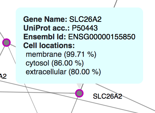
Download the PPI network
By clicking on the download button, which is present just above the network module, you can download it in its current state, in the Graph ML format. This file format can be imported in various graphical tools, e.g. with yED or in network analysis tools, such as Cytoscape and and Gephi.

Cellular information

At the right panel of this section you can explore the cellular location of all proteins present in the PPI network, with the interactive cellular location pie chart. Each part of the chart corresponds to a different cellular location.

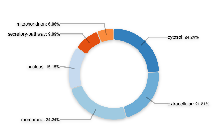
You can:

Hover over a cellular location
By hovering on a particular cellular location you can get further statistics inside the plot for the:
- Ratio of the location: number of protein-cellular location links among all protein-cellular location links
- Overlap ratio of the location: number of proteins present in the cellular location among all proteins of the network
All proteins of the PPI network that belong to this location will be automatically coloured as well.

Pathway information

In this section you can explore the cellular pathways where the genes in your selected module are involved in with the summary pathway treemap on the left panel and the detailed pathway table on the right panel.

All required information is extracted from Reactome.

Pathway treemap

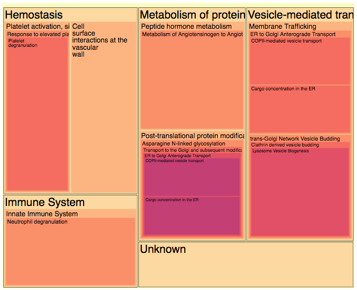
The treemap on the left panel of this section shows the summary of the different pathway categories of the genes present in your selected gene module.

Each main pathway category is enclosed in a box surrounded by a black stroke and contains nested pathway subcategories, based on the information from Reactome, descending from the more general to the more specific ones. The last sub-category is the most detailed pathway mapping of the gene.

The ordering from the more general to the more specific pathway categories is shown with a transition from:

bigger to smaller text font
lighter to darker colour gradient

The size of each main pathway category is determined by the number of genes of the selected module that it contains.

Pathway table

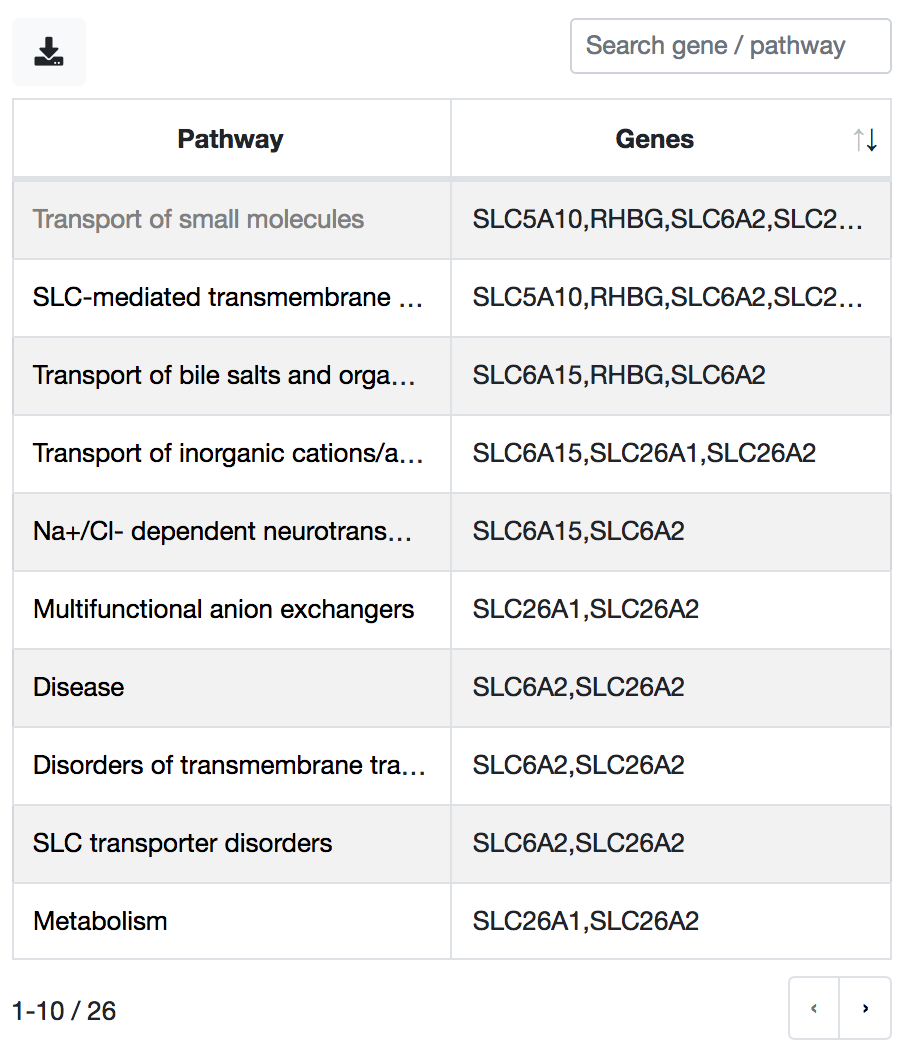
The pathway table shows more details about all pathway categories (general and specific) of your gene module.

You can:

order the appearance of the pathways based on the number of your module genes they contain.
click on each pathway to get further information from its corresponding page in Reactome.
search/filter the table based on a pathway or gene name(s). You can provide multiple gene names, separated with space.
download the table with the button.

NOTE: if you select to download the pathway table while you have an active gene/pathway search, only the information about the filtered table will be downloaded. Therefore, if you want to download the complete table, you should make sure that the search field of the table is empty.

Gene pair ranking exploration

With this section you can explore the gene pairs that are present in your data and rank them based on the content of candidate disease-causing variant combinations that have been predicted with VarCoPP.

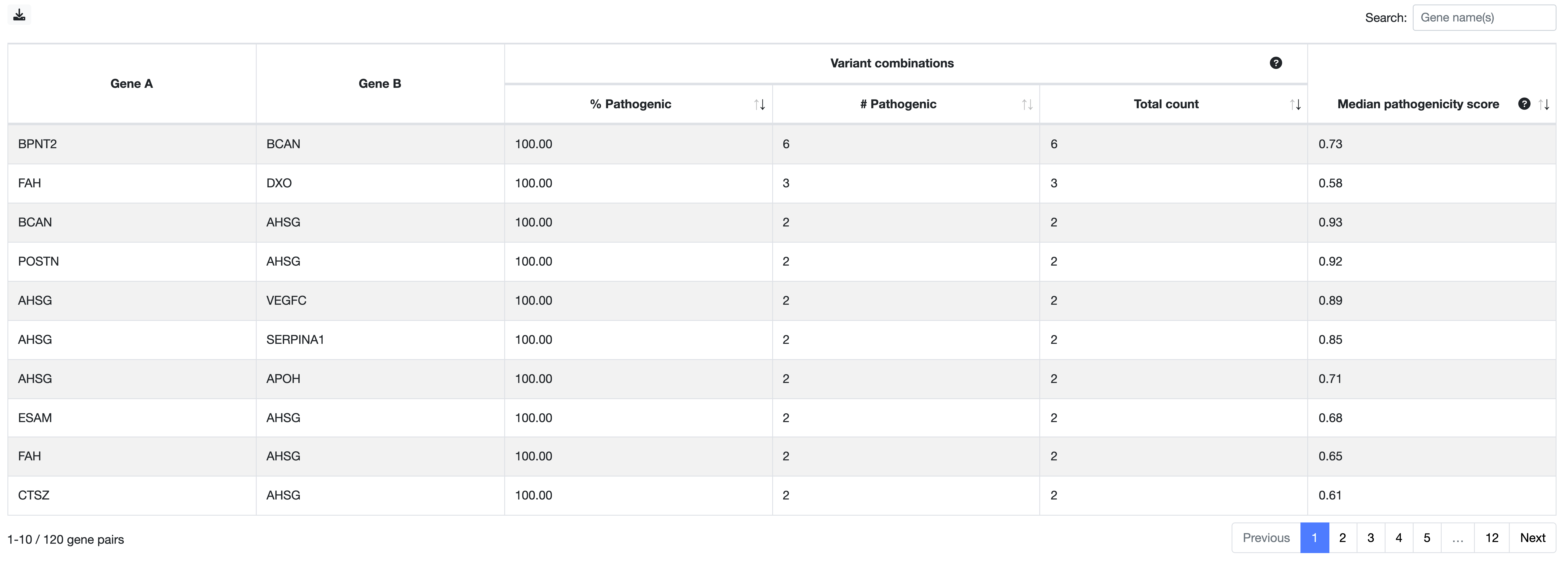
This information is shown in a gene pair table that provides statistics on all gene pairs present in your data. The table is divided into the statistics on the percentage and number of pathogenic variant combinations for each pair, and the pathogenic score provided by VarCoPP among combinations of that pair, to get an idea of their severity.
For further explanations on how this pathogenicity score is calculated, you can consult the VarCoPP section on this Documentation page.

The table is initially ranked based on the following columns in descending order of importance:

percentage of pathogenic combinations
VarCoPP Score

You can:

Rank the table based on a column:
You can rank your table based on a column by clicking on the arrows on the column name.
Search/filter the table based on gene(s):
You can search for a gene by typing the gene name in the search area.
You can also search for a gene pair by typing the two genes you are searching, separated with a space.
Download the table:
You can download the current table by clicking on the button. If you have filtered first your table based on a gene, the downloaded table will only contain that selection.

NOTE: the genes inside each gene pair are ordered according to their Residual Variation Intolerance Score (RVIS). For each pair, gene A is always the gene with the lowest RVIS and, thus, with a higher probability to carry damaging mutations. For more information on the gene ordering and the creation of digenic combinations, you can consult the Creating digenic combinations section in the Documentation page.

NOTE: if you want to download the gene pair table while you have an active search/filter based on gene name(s), only the filtered table will be downloaded. You can re-initialize the gene pair table, by removing the gene name from the search area.

Digenic combinations exploration

With this section you can explore the results of the digenic pathogenicity predictions of VarCoPP for all digenic variant combinations of your data.

You can get a visual overview of the results with the interactive Swarm plot and inspect and download all results with the Summary table. By clicking on each digenic combination in the table you can get more details about its pathogenicity prediction, its pathogenic digenic effect and get access to useful variant, gene and gene-pair annotations.

Digenic results overview: swarm plot

The swarm plot gives an interactive visual overview of the VarCoPP predictions for all digenic variant combinations present in your data.

NOTE: The swarm plot can not be properly displayed for large amounts of data (> 10,000 variant combinations). In that case, a reduced version of the plot is shown where the jitter is removed, since it does not allow for visualization of all data points.

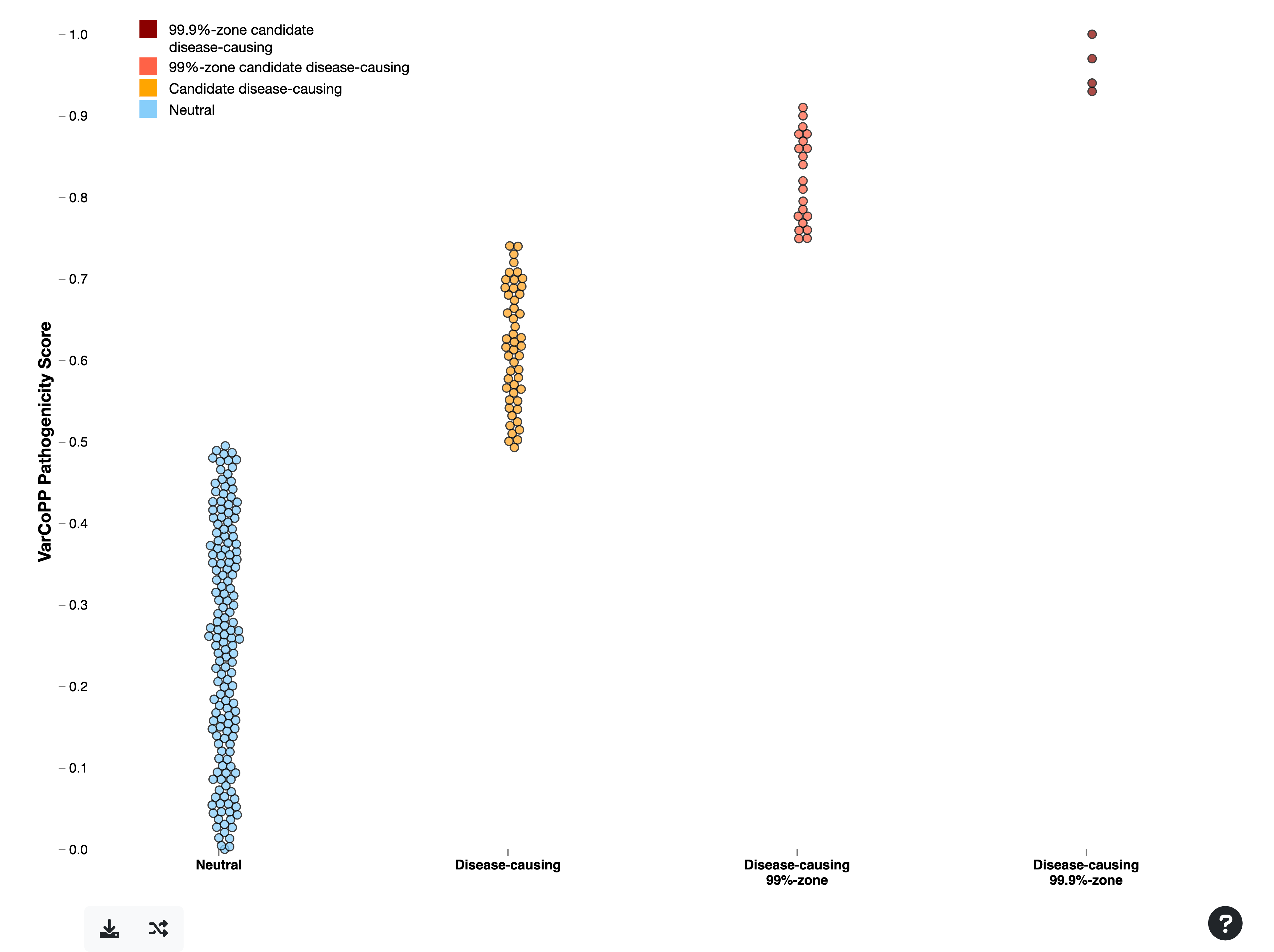
All combinations are plotted based on their prediction score and the pathogenicity confidence that is provided with VarCoPP for that combination (for details on how this confidence is calculated, you can consult the VarCoPP confidence zones section in the Documentation).

dark red

the variant combination is predicted as candidate disease-causing with 99.9% confidence

red

the variant combination is predicted as candidate disease-causing with 99% confidence

orange

the variant combination is predicted as candidate disease-causing without falling into one of the two confidence zones

blue

the variant combination is predicted as neutral

A graphical summary of the distribution of variant combinations in these confidence zones is shown above the swarm plot.

You can interact with the plot in several ways:

Hover on a combination:
By hovering on a combination in the plot, a box appears with information about the gene pair, the VarCoPP pathogenicity scores and further links.
Download the plot:
You can download the plot by clicking on the button.
Add extra jitter to the plot:
You can add jitter to the plot by clicking on the button.

Digenic results overview: Summary table

The summary table on the right panel shows further details for each digenic combination. That table is automatically updated based on the filters you choose on the table itself.

The combinations are ranked based on their VarCoPP Score, with those having the highest score being first.

You can:

click on each digenic combination to get more details about its pathogenicity prediction, its pathogenic digenic effect and get access to useful variant, gene and gene-pair annotations.
search/filter the table based on a variant or gene name(s). You can use multiple variants or genes by separating them with a space.
download the table in its current state by clicking on the button.

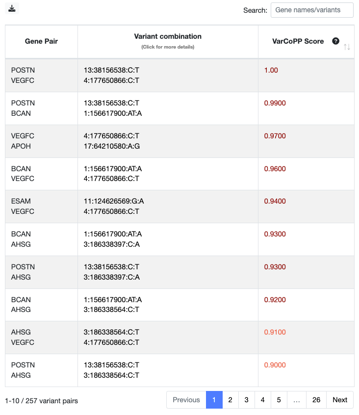
NOTE: if you want to download the variant combinations table while you have an active search/filter on the table, only the table corresponding to those filters will be downloaded. You can re-initialize the table, by removing the genes/variants from the search area.

The colour of each digenic combination in the table represents the pathogenicity confidence of the combination (for details on how this confidence is calculated, you can consult the VarCoPP confidence zones section in the Documentation).

dark red

the variant combination is predicted as candidate disease-causing with 99.9% confidence

red

the variant combination is predicted as candidate disease-causing with 99% confidence

orange

the variant combination is predicted as candidate disease-causing without falling into one of the two confidence zones

blue

the variant combination is predicted as neutral

Pathogenicity prediction information

In this section you can explore the results of VarCoPP, which predicts the pathogenicity of a digenic variant combination as either candidate disease-causing or neutral. Furthermore, you can see further explanations on how each biological feature decides for either the disease-causing or the neutral class. This is an important step that can aid in understanding and evaluating the results obtained by our predictive methods.

In ORVAL we are using the tree-interpreter python module, a method that allows us to see, for every variant combination, the preference each feature shows for either the neutral or the disease-causing class inside the VarCoPP predictor. Based on this method, we get specific preference values for each feature that range from negative to positive.

We visualise these class preference values per feature by using bar plots that reveal both the class preferences in VarCoPP.

Feature in red color

The feature has a positive preference value and votes in favor of the disease-causing class. The higher the value, the stronger the vote for the disease-causing class is.

Feature in blue color

The feature has a negative preference value and votes in favor of the neutral class. The lower the value, the stronger the vote for the neutral class is.

For a detailed description of the biological features used for predictions, you can consult the VarCoPP features section.

NOTE: the feature preference values shown in the boxplot do not correspond to the real values of the features. They are specific values that are collected during our analysis and only show the preference of each feature to either the disease-causing or neutral class.
You can consult the real values of the features in the Annotations section of the digenic combination page.

An example of feature interpretation for a prediction

The following barplot corresponds to a bi-locus combination that was predicted as candidate disease-causing with a VarCoPP Score of 0.88.

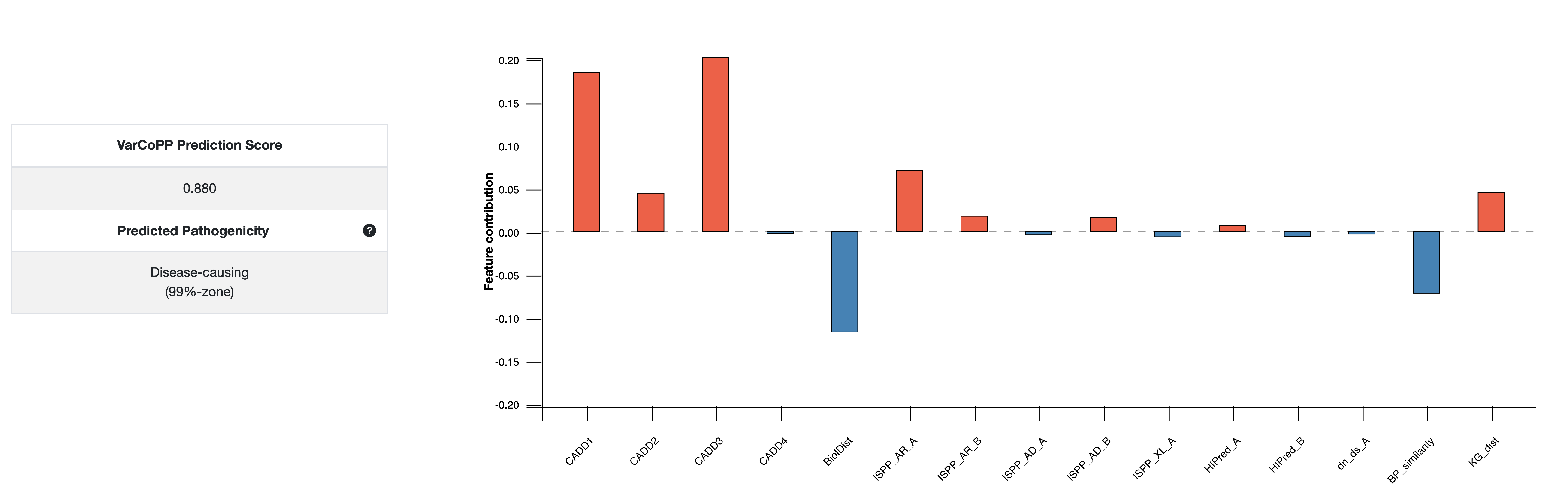
In the barplot, we see the preference of each feature for either the disease-causing or the neutral class among all individual predictors of VarCoPP, for that particular variant combination.

In this case, we can see that CADD1 and CADD3 (the CADD scores of the 1st variant allele of gene A and B, see also the Feature Description section), contribute a lot to the disease-causing class vote, as they have the highest positive contribution median value among the rest of the features. This probably means that the CADD scores of those variant alleles are quite high, something that we can verify by looking at the annotation of the digenic combination in the Digenic Results page.
On the other hand, BiolDist (the biological distance between gene A and gene B) drives the prediction towards the neutral class.

Digenic Effect prediction

In this section you can explore the results of the Digenic Effect (DE) predictor that predicts the digenic effect of a pathogenic variant combination (i.e. whether it is True Digenic, Monogenic + Modifier or a Dual Molecular Diagnosis case). If a variant combination has been predicted as candidate disease-causing, you will find further information of its digenic effect in this section.

This information is presented on the left with a table that provides the probabilities for each digenic effect class and the predicted Digenic Effect (i.e. the class with the highest probability), while the radar plot on the right panel provides a visual representation of the prediction results.

An example of a Digenic Effect prediction

The following image corresponds to a pathogenic variant combination whose digenic effect is predicted to be True Digenic.

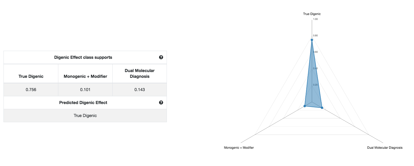
example of a digenic effect prediction for a combination

The table on the left provides the probabilities for all three possible digenic effect classes. We can see that the True Digenic class has the highest probability (0.756) compared to the rest and, therefore, this is the final Digenic Effect class that is predicted for that combination.

The radar plot on the right simply shows a summary visualisation of the results shown in the table. Each line represents a Digenic Effect class and can take probability values from 0 (center of the plot) to 1 (edge of the plot). Three dots fall to the corresponding probability value of each class respectively, forming a triangular shape. With this shape we can get a quick visual idea of which class is prefered and whether this preference is strong or not (depending on the skewness of the triangular shape). In this case, we can clearly see that the prediction falls to the True Digenic class based on the skewness of the triangular shape towards this class.

Exception messages

In some cases you will not be able to get information about the Digenic Effect of a variant combination and you will see some exceptional messages instead:

The variant combination is not pathogenic
As the Digenic Effect predictor can only work on pathogenic variant combinations, if the combination you are exploring is predicted as neutral by VarCoPP, you will see the following message:
There is some missing annotation for a variant combination
The Digenic Effect predictor cannot make a prediction for a variant combination when some annotations that are used for the prediction are missing for that combination. In this case, you will see the following message:

Tutorials

In case you would like to see a specific tutorial in ORVAL, you can contact us.

Prioritisation of digenic variant combinations

Depending on the size of the data you are analysing you may end up with many digenic variant combinations predicted as candidate disease-causing. ORVAL is not a prioritisation tool per se, however, it is possible to limit your analysis to those combinations that could potentially be more interesting for your research. For this, you can follow the next steps:

1. Overview and filtering of the digenic variant combinations

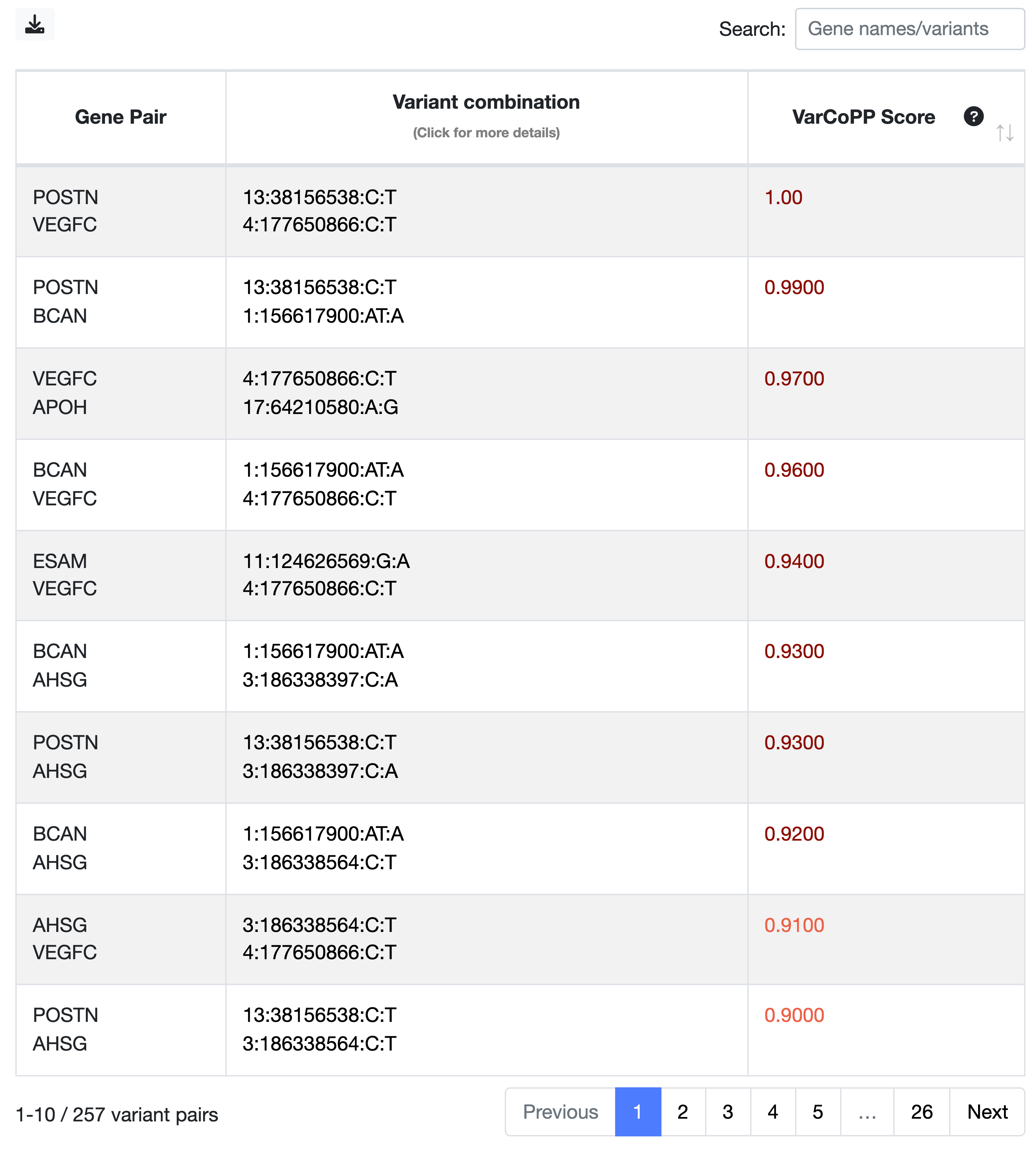
The combinations in the Summary Table are ranked based on their VarCoPP scores, with those at the top having the highest scores. The higher the score assigned to a digenic combination, the more confident VarCoPP is for the disease-causing class (consult the VarCoPP section for a detailed explanation).

The strictest way to filter your combinations is by focusing on those falling in the 99.9%-confidence zone, in dark red colour (the first two combinations in this example). These have 0.1% probability of being False Positives. Keep in mind that this selection can be quite strict and can lead to False Negatives.
To lessen your criteria, you can also include the combinations falling in the 99%-confidence zone in red colour (the next five combinations in this example), which have 1% probability of being FPs.
If the steps described below do not yield convincing results, you can also try to include the combinations that are predicted as disease-causing but do not fall in any of the two confidence zones, and these are depicted in orange.

For more information, consult the VarCoPP Confidence Zones section of our Documentation page.

2. Find relevant gene modules in the predicted pathogenic gene network

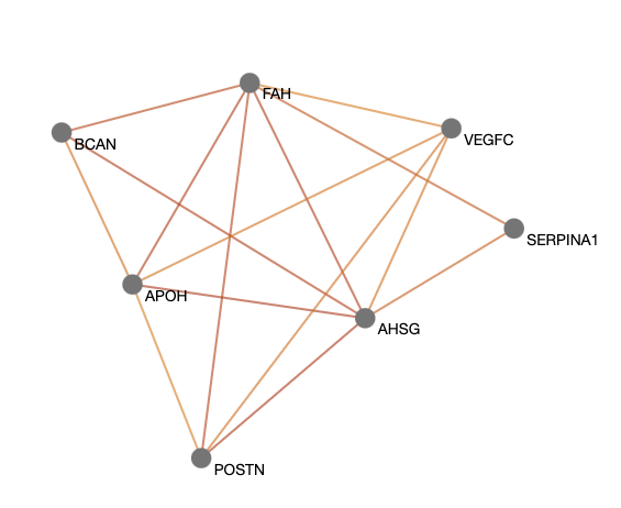
Are the genes relevant? You can explore the predicted pathogenic gene network in ORVAL, which appears first in the results page. In this network, two genes are connected with an edge only if they contain at least one predicted pathogenic digenic combination.

You can first filter the network to keep the most relevant gene pairs, based on the pathogenicity cutoff that you choose. You can use the Filtering panel on the left, to keep only the gene pairs containing combinations falling in the 99%- and 99.9%-confidence zones, by selecting 0.74 (hg19) or 0.65 (hg38) as the minimum Gene Pair Pathogenicity Score threshold (i.e., this is the minimum VarCoPP Score for the 99%-confidence zone, see the VarCoPP Confidence Zones section of our Documentation page).
For a stricter analysis, you can use the 0.89 (hg19) or 0.85 (hg38) value as a cutoff to include only gene pairs with combinations falling in the 99.9%-confidence zone.

Once you are satisfied with your network, click on a gene in the network to make the gene module panel appear on the right and click on the link that appears to get directed to another page the shows PPI and pathway information for those genes.

NOTE: if a gene is shown as a hub in the gene network, meaning that it is highly connected with other genes, it may mean that it contains a variant there that drives the predictions higher. This may indicate that a Monogenic plus Modifier concept may be present in your data. However, if this gene does not seem relevant for the phenotype or seems unrelated to the rest of the genes, you could try to remove it from the network and consider the rest of the genes. You can use a general Centrality threshold of your choice or unselect genes manually in the gene table on the left.

Detailed information on ways to filter your network can be found in the Oligogenic network section of our Documentation.

3. Explore the relationship between the genes in the gene module

Once you click on the gene module link, ORVAL offers PPI, cellular location and molecular pathway information as a starting (and definitely not exhaustive) point to understand the relevance and interactions of genes in-silico. For an explanation of these graphs, consult the Oligogenic gene module, PPI network and Pathway information sections of our Documentation.

Are the genes in your module related in terms of their PPIs? In the PPI network (the first picture in this example) you can see whether the proteins of this module (purple nodes) directly interact (purple edges) or indirectly interact with one external protein in between, which are depicted as grey nodes and are linked with grey edges. In this example, the proteins of your module TRIM54 and TRIM63 directly interact, but also indirectly interact with several other external proteins found in the comPPI database.

Are the genes in your module involved in similar molecular pathways? You can consult the Reactome pathway treemap and the pathway table to find genes involved in similar pathways (the second picture in this example).

This is a starting point for you to explore the relationships between the genes present in the selected module. Based on this information, you can start limiting the results to the gene pairs that seem to be most relevant.

4. Explore the variant combinations of the selected gene pairs

example of a boxplot explaining the voting preference of VarCoPP features

example of the digenic effect prediction

You can now go back to the digenic variant combinations Summary Table (first picture) and the Swarm plot, and explore the variant combinations that are linked to the gene pairs that you have selected based on the previous steps. Especially if multiple variant combinations are linked with the same gene pair, it will be interesting to further explore their predictions to see which are relevant. A summary statistics for each gene pair is also available at the Gene pair ranking table of the Main Results page.

Once you find a combination of interest, you can click on it in the Summary Table (second column) or in the Swarm plot, and you will be directed to a page with information specific for that combination. There, you can first see a summary of the variants and the predictions of both VarCoPP and the Digenic Effect predictor.

You can explore the Feature preference boxplot of VarCoPP (second picture). How do the features vote for either the disease-causing (features in red colour), or neutral (features in blue colour) class? The more these feature preferences deviate from zero, the stronger their vote for a particular class is. In this example, we see that the CADD score of the variant alleles of gene A (CADD1 and CADD2) vote the strongest for the the disease-causing, whereas the CADD score of the first variant allele of gene B (CADD3), as well as its recessiveness probability (RecB) vote the strongest for the neutral class. You can further evaluate the values of these features and why they tend to vote for either class in the Annotations section of that page.

You can further get an indication of the Digenic Effect of that particular combination, i.e. whether it has a True Digenic, Monogenic gene plus Modifier or Dual Molecular Diagnosis effect (third picture). These predictions are indicative and further inspection or confirmation is required. In this example, the variant combination has a very strong prediction for the True Digenic class.

The information in this page can help you evaluate whether the specific variant combination seems relevant for your analysis.

5. Examine the relevance of selected gene pairs and combinations for the phenotype

Do the selected gene pairs and variant combinations make sense to you as a clinical researcher and are they in accordance or could they explain the patient's phenotype? At this step, you have a filtered set of gene pairs and variant combinations that could be potentially relevant, based on in silico information.

6. Optional: Repeat steps 1-5 with less strict criteria

If at this point the information seems incomplete or you still do not obtain promising results, you could lessen the strictness of your criteria and repeat the steps 1-5. For example, if you have selected only gene pairs with combinations falling into the 99%-confidence zone, you could now also allow gene pairs with combinations falling also into the 99%-confidence zone. Furthermore, if combinations falling into these confidence zones are not available or they do not seem convincing, you can try to include all gene pairs and variant combinations predicted as disease-causing.

7. Explore familial and functional evidence

The previous steps provide a way to limit your analysis to those variant combinations that seem to be more relevant or more promising for further research and experiments. ORVAL cannot, in any way, provide a definite way for diagnosis or medical advice. Further evidence is needed to show whether they can indeed be True Positives based on segregation analyses and functional experiments.

Browser compatibility

You can find below which browsers are suitable for ORVAL based on your operational system:

OS	Version	Chrome	Firefox	Microsoft Edge	Safari
Linux	Ubuntu 20.04	100.0.48	99.0	N/A	N/A
MacOS	Monterey	100.0.48	99.0	N/A	15.4
Windows	10/11	100.0.48	99.0	100	N/A

Frequently Asked Questions

If answers to your questions are not provided in this section and no information about your question is mentioned in the Documentation page, you can contact us.

Is there a limit on the number of variants I can uploaded?
In general, we highly recommend the use of variants from up to 300 genes, as well as the application of the variant filtering procedure that is provided with ORVAL, in order to limit the amount non-relevant combinations that will be tested.

Based on our server testings, you can either copy-paste a variant list of up to 80000 variants or upload a VCF file of size up to 50 MB. You can consult the Input Data section of our Documentation page for more details.

Can I include variants from multiple patients in my input?
No, the analysis should be restricted to a single individual only, as ORVAL creates all possible variant combinations from your variant list assuming that they belong to the same person.
If you want to analyse multiple patients, you should separate their variants in different files and explore them individually with ORVAL.

Is there a specific input format for the insertions and deletions?
ORVAL accepts different types of variant format for the insertions and deletions, involving dashes or not.
You can consult the Variant Types section in the Documentation page for a detailed explanation.

I see that the Job status of my variant submission is FAILURE. What should I do?

If there is no specific error message that explains the problem, you can follow these steps:

Check if your internet connection is running smoothly.
Re-try your data submission.
Check if your input data is correctly formatted. You can consult the Input Data section in our documentation page for a detailed explanation on the correct format for your variant submission.

If you have checked the previous steps and you still experience issues, you can send us an email, providing also the Job Id you have obtained during the submission.

During my data submission I see a message that I have exceeded the 5 Job submissions. What should I do?

For server monitoring purposes we allow every user (based on their IP address) to run maximum 5 different data analyses at the same time. In case you exceed this number, you have to wait until at least one of the running jobs is finished to launch a new one. You can consult the Job Submission section of the Documentation page for more details.

During my data submission I see a message that my uploaded file is using an unsupported format. What should I do?

The VCF file you have uploaded is not correctly formatted and ORVAL cannot parse it. Make sure that your file contains the header line (#CHROM POS REF ALT etc...) and tab-delimited columns with the CHROM, POS, ID, REF, ALT, FORMAT, SAMPLE_NAME columns.
You can consult the VCF file specification section of the Documentation page for a detailed description on how to properly format your VCF file.

What types of digenic combinations does ORVAL create?
ORVAL creates all possible di-allelic, tri-allelic and tetra-llelic variant combinations between any gene pair present in your data, including heterozygous compound variants in one of the two genes. Tetra-llelic combinations with four heterozygous variants (two in each gene) are not created, as these combinations were absent from our training set.
For a detailed explanation, you can consult the Creating digenic combinations section of our Documentation page.

I receive an error message that there are no variant combinations left to do the analysis. What should I do?

You can check the following steps to explore possible solutions:

Check whether the selected genome version is correct. ORVAL can annotate variants using the GRCh37/hg19 or GRCh38/hg38 genome version, see the Genome version section of the Documentation page for more details.
Try to relax your variant or gene filtering options, especially the option for removing intronic and synonymous variants.
Ensure that you have more than one genes present in your data. ORVAL makes variant combinations between gene pairs, so it requires the presence of at least two different genes in your data.
If you have submitted a small number of variants, these variants may have been excluded from the analysis during the annotation process. For example, the CADD score for those variants may be missing, and as this score is important for the predictions, variants without an annotated CADD score are excluded from the analysis. A detailed list of all possible cases where your variants may be excluded is presented in the Variant Exclusion section of the Documentation page

If you have checked the previous steps and you still experience issues, you can send us an email, providing also the Job Id you have obtained during the submission.

SOME variants of my initial submission are missing from the results

Please check the variant and/or gene filtering options you have selected during your submission, as these play an important role on the absence of some of your variants in the analysis. The variant filtering options offered by ORVAL are automatically pre-selected during the submission, unless you unselect them.
Make sure that the variant information and format you provided is correct for all variants. In case you copy-pasted a variant list using the box panel, make sure that the zygosity values are not misspelled (Heterozygous or Homozygous zygosity values are accepted), see also the tab-delimited variant list section in the Documentation page.
Otherwise, some variants may have been excluded from your analysis during the data annotation process. You can consult the Variant Exclusion section of our Documentation page for a detailed description of such cases.

For more information regarding our filtering options and the data annotation process, you can consult the Data Filtering and Annotation section of our Documentation page.

I am pretty sure that a variant is supposed to be mapped to a specific gene (according to my knowledge or the gene panel I provided), but I see another gene name instead in the results.

This can happen for the following reasons:

The gene symbol present at the gene panel file is not the official HGNC gene symbol. During annotation we only use the official HGNC gene symbols, and thus, we will display this symbol instead of the one that you provided.
The position of the variant for that gene overlaps with other genes. In this tricky situation, we have to choose one gene to continue with predictions. We have developed a set of priority rules for that (see the Gene annotation section). Therefore, there is a chance that we have assigned this variant to another gene instead. Unfortunately, it is not possible to re-assign it to your favourite gene manually and we can potentially do changes in our database for that only during major ORVAL updates. Please note that you shouldn't change that gene name for the variant in the results, as some prediction features are gene-specific.
If you think that this mapping is definitely wrong, you can send us an email.

I cannot see a network in the Results page
You can see a network in the Results page only if there is at least one candidate disease-causing variant combination predicted with VarCoPP, see for more details the Network navigation section in the Documentation page.
In any case, you can still explore all variant combinations in the Digenic predictions of the Results page.

Why do we see only SOME external proteins in the PPI network?
You see an external protein in the PPI network only if it links two proteins of your selected module with a direct protein-protein interaction. External proteins that are connected with your module proteins with higher degrees of interactions are not shown. You can consult the PPI network exploration section in the Documentation page.

Where can I find the Digenic Effect prediction for a variant combination?
You can see the Digenic Effect prediction of a variant combination on their corresponding Digenic Combination page. You can get directed to this page by clicking on a variant combination either in the Digenic Combinations Overview table or on the Swarm plot.
Please note that you will only see a Digenic Effect prediction if the variant combination is predicted as pathogenic with VarCoPP.

Do you store any of my data?
We store the results of your data submission for 7 days, so that you can re-access the corresponding Result pages. After this period, all data is deleted.
We do not store email addresses that you may have provided to us during the data submission. However, we track general user traffic information (e.g. IP addresses) for job monitoring purposes (e.g. restricting the number of parallel submissions from the same ID address).
For a detailed explanation of our Data Privacy procedures, you can consult the Data privacy section of the About page.